Below, I run a power analysis for Study 1 in Dietvorst, Simmons and Massey’s (2015) paper on algorithm aversion. The experiment tested the hypothesis that “seeing the model perform, and therefore err, would decrease participants’ tendency to bet on it rather than the human forecaster, despite the fact that the model was more accurate than the human.”
Experimental participants were given a judgment task, with one group allowed to see the algorithm in action before undertaking the task. Participants were given the option of using the algorithm’s predictions or their own. Those who had seen the algorithm perform were less likely to use it in the task.
First I run a power analysis using data from the original experiment. Post-experiment power analysis should not be done to justify the sample size in the original study, as any significant effect in an underpowered study is likely to be exaggerated in magnitude. If you then use this exaggerated effect to calculate power, it may give the impression that the experiment was adequately powered.
However, this post-experiment analysis may still provide some information about the study’s robustness. It also provides a starting point for further analysis where we adjust the effect size within a plausible range to test how sensitive the assessment of power is to the effect size.
To calculate power, we need to know the sample size (per group) and the proportion choosing the model in each group.
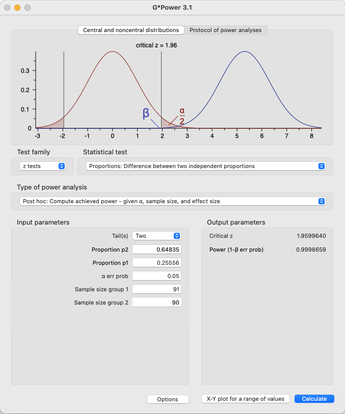
In Dietvorst et al (2015) Study 1, the smallest group had 90 members. In those groups, 59 of 91 in the control group chose the model, and 23 of 90 who had seen the model perform chose the model.
I will use the R command power.prop.test to do these calculations. That function requires that we provide all except one of the number of observations per group (n), the probability in one group (p1), the probability in the other group (p2), the power of the test and the significance level. The function then calculates the left-out parameter.
The power of that comparison was:
Code
power.prop.test(n=90, p1=59/91, p2=23/90)
     Two-sample comparison of proportions power calculation

              n = 90
             p1 = 0.6483516
             p2 = 0.2555556
      sig.level = 0.05
          power = 0.9998577
    alternative = two.sided

NOTE: n is number in *each* group
A alternative is to use the pwrss package. You can use the pwrss package either directly via the R command line or using this Shiny app-based website.
In G*Power, we select the type of test that was conducted (z-test, difference between two independent proportions) and select the analysis as a post hoc calculation of achieved power. Pressing calculate gives us the result and a graph of the distributions.
The power of the test was over 99.9%.
However, this effect size may not be representative. The other studies in Dietvorst et al (2015) had smaller effect sizes, as did the replication of Study 3b by Jung and Seiter (2021).
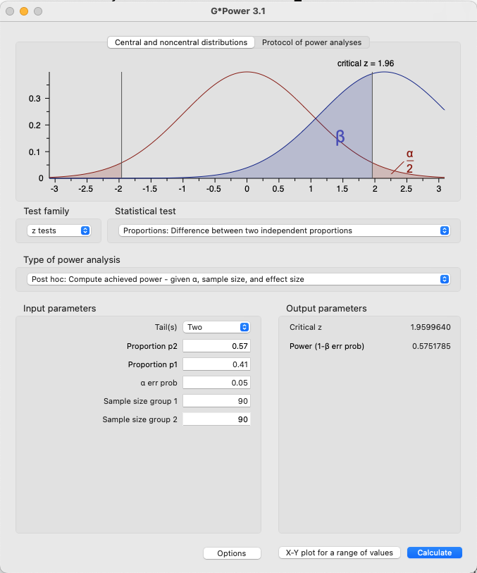
The effect size of Dietvorst et al (2015) Study 3a was 16%, with 57% in the control and 41% in the model group choosing the model. Assuming that is the true effect size in Study 1, we would have the following power.
     Two-sample comparison of proportions power calculation

              n = 90
             p1 = 0.57
             p2 = 0.41
      sig.level = 0.05
          power = 0.5751626
    alternative = two.sided

NOTE: n is number in *each* group
If that effect size was the true effect size, that gives only 57% power.
Similarly, Jung and Seiter (2021) found that 67% of the control group and 47% of the treatment group chose the model. This is a smaller effect size than Study 1, but larger than that is Study 3b of Dietvorst et al. Again, if we assumed that is the true effect size in Study 1, we would have the following power.
     Two-sample comparison of proportions power calculation

              n = 90
             p1 = 0.67
             p2 = 0.47
      sig.level = 0.05
          power = 0.7780998
    alternative = two.sided

NOTE: n is number in *each* group
This results in a power of 77%, which is below the common “rule of thumb” of 80% power.
For caution, let us assume that the smallest effect size, that in Dietvorst et al (2015) Study 3a is representative of the true effect size for Study 1. We can then calculate the sample size required to achieve 90% power as:
Here I again use the R command power.prop.test, but in this case specify the desired power such that the function outputs the required sample size.
Code
power.prop.test(p1=0.57, p2=0.41, power=0.9)
     Two-sample comparison of proportions power calculation

              n = 203.0558
             p1 = 0.57
             p2 = 0.41
      sig.level = 0.05
          power = 0.9
    alternative = two.sided

NOTE: n is number in *each* group
Ninety per cent power would require a sample of 200.
Dietvorst, B. J., Simmons, J. P., and Massey, C. (2015). Algorithm aversion: People erroneously avoid algorithms after seeing them err. Journal of Experimental Psychology: General, 144, 114–126. https://doi.org/10.1037/xge0000033
Jung, M., and Seiter, M. (2021). Towards a better understanding on mitigating algorithm aversion in forecasting: An experimental study. Journal of Management Control, 32(4), 495–516. https://doi.org/10.1007/s00187-021-00326-3